


Alvarez, F., Le Bihan, H. & Lippi, F. (2014) “Modelling sticky prices and the effect of monetary shocks“, VoxEU Organisation, 30 September.
The assumption of sticky prices is central in understanding the effect of monetary policies on the economy. Yet, how to best model price stickiness is an unresolved issue. This column assesses a selection of models that are able to reproduce cross-sectional heterogeneity in the setting of prices. The authors derive a formula which gives a useful approximation of the effect of a small monetary shock on total output. The formula demonstrates the importance of the Kurtosis of the distribution of price changes. It can be applied to a large class of models, including such with different timing of price adjustment.
Most macroeconomic models embed some form of sticky prices, i.e. inertia in price-setting decisions. The main motivation for sticky prices is the empirical observation that individual good prices tend to remain fixed for long periods of time, typically a few months for CPI items. The sticky prices assumption is central in understanding how monetary policy actions propagate the macro economy; absent sticky prices, standard models predict that monetary policy is irrelevant for the dynamics of output and other real variables.
Modelling sticky prices
Yet, how to best model price stickiness is an unresolved issue with relevant macroeconomic consequences. Depending on the details of how stickiness is modelled, the effects of monetary shocks range from negligible to substantial. Examples include:
- The Taylor model, in which firms keep prices unchanged for a fixed period of time (say six months);
- The menu cost model, according to which firms explicitly incur a cost for changing prices (for instance, the physical cost of changing the price sticker), and select the timing of their changes in prices weighing the costs and benefits of inaction.
- The Calvo model, in which there is a constant fixed probability of changing the price, independent of the economic environment, and of time since the last price change.
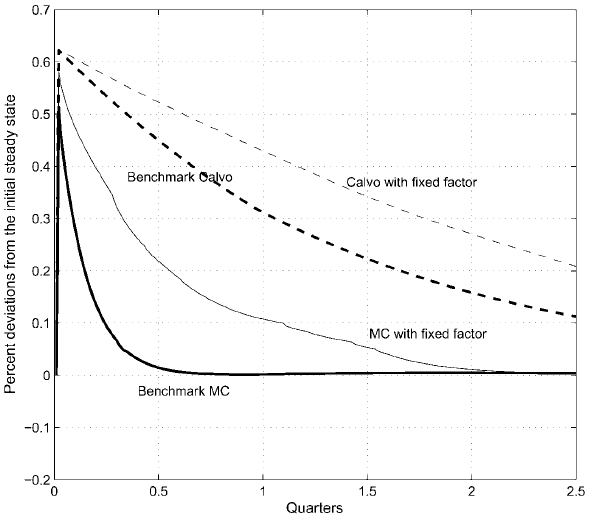
Figure 1 below, taken from an influential paper by Golosov and Lucas (2007), illustrates that different modelling assumptions, consistent with the same firm-level price stickiness (say two price changes per year), imply large differences in the response of the aggregate economy to monetary shocks. Each curve plots the response of GDP as a function of time after a monetary shock — a 1% increase in money supply in their analysis. The solid blue curve corresponds to a menu cost model; the red dashed curve corresponds to a Calvo model. We stress that both models produce a frequency of price adjustment, so they have the same ‘price stickiness’. Yet, the effects on GDP are very different. The total amount of extra GDP that the economy produces after the monetary shock, as given by the area under the curve, illustrates this point. In the case of Calvo, the order of magnitude of the cumulative response is around 0.5% of GDP. In the menu cost model, the cumulative output effect is smaller (about 6 times) than in the Calvo model.
Figure 1. Output response to monetary shock in the menu cost versus the Calvo model
Relevant posts:
- Petralias, A. & Prodromídis, P. (2014) “Price discovery under crisis: Uncovering the determinant factors of prices using efficient Bayesian model selection methods“, Crisis Observatory, 28 July.
- Kahn, R. (2014) “Lowflation: Should We Fear Stable Prices?“, Global Economics Monthly: June 2014, Council on Foreign Relations, 10 June.
- Fatas, A. (2014) “The Price is Wrong“, Antonio Fatas on the Global Economy Blog, 14 April.